Using The Solver Viewer¶

The Solver Viewer is a graphical tool for loading motion-planning scenes, selecting and configuring solvers, running them, and visualizing the resulting paths and roadmap graphs. It is the primary tool for interacting with and evaluating any solver written for DiscoPygal.

This guide covers every panel, toolbar action, and display option so that you can go from a raw scene file to an animated solution in a single session.

The toolbar icons shown below come from the Solver Viewer resource folder.

Prerequisites¶

Complete:

Prerequisites
Discopygal Installation
Build a scene with the Scene Designer, or use one of the bundled example scenes.

Step 1: Launch the Solver Viewer¶

Activate your virtual environment and start the tool.

source .venv/bin/activate
solver_viewer

.\.venv\Scripts\Activate.ps1
solver_viewer.exe

The window opens with an empty canvas titled “DiscoPygal Solver Viewer”. You can also pass a scene and solver directly at launch — see Command-line usage below.

Step 2: Understand What the Viewer Manages¶

The solver viewer works with three kinds of data at runtime.

The scene¶

A scene is loaded from a JSON file (or passed in as a Scene object from a script). It contains the workspace geometry, robot definitions, and start/goal configurations. The path to the currently loaded scene is shown read-only in the top bar. Once a scene is loaded, its metadata — version, recommended solvers, and description — appears in the properties panel on the right.

The solver¶

A solver is a class that inherits from Solver. Built-in solvers are registered automatically at startup. Additional solvers can be imported from any Python file at any time. When a solver is selected, its configurable parameters appear as labelled text fields in the left-hand panel. The solver’s class name is shown in the Solver label at the top of that panel.

The solution¶

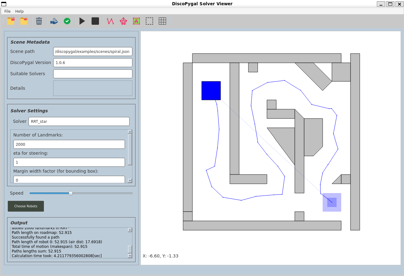
After a solver runs successfully, the viewer holds the computed paths, the roadmap graph, an optional CGAL arrangement, and an optional bounding-box graph. Each of these can be toggled on and off independently in the canvas.

Step 3: Tour the User Interface¶

solver settings¶

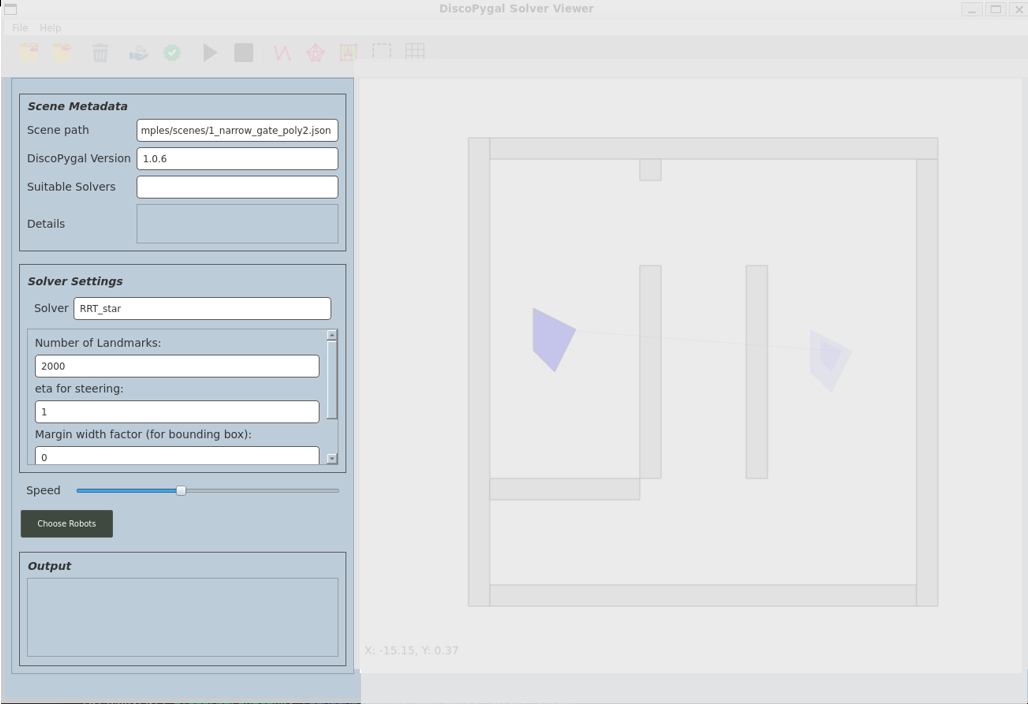
When a solver is selected, its parameters are generated dynamically in the left-hand panel as a scrollable list of labelled text fields. Each field shows the parameter’s description and its current value. Edit any field before clicking Solve to override the default. The panel is scrollable when a solver has many parameters.

scene metadata¶

After a scene is loaded, the right-hand panel shows three read-only fields drawn directly from the scene’s JSON metadata:

Field	Content
`version`	The DiscoPygal version that created the scene.
`solvers`	Solver class names recommended for this scene.
`scene details`	Human-readable description of the scene.

Log panel¶

A text area at the bottom of the window receives all messages written by the solver via its log() method, including progress updates and the total calculation time reported at the end of every run.

Choose Robots panel¶

Clicking the Choose Robots button reveals a scrollable list of checkboxes, one per robot in the loaded scene. This panel is hidden until a scene is loaded. See Step 9: Filter by Robot for details.

Speed slider¶

The horizontal slider below the toolbar controls animation playback speed. Moving it takes effect immediately, adjusting the duration of every remaining animation step proportionally — even while the animation is playing.

Canvas¶

The large central area renders the scene, overlays, and animated robots. Moving the mouse over the canvas shows the current scene coordinates in a small floating label. Double-clicking also updates the coordinate display.

Step 4: Load a Scene¶

Click Open Scene in the toolbar, or use File → Open Scene, and select a .json scene file. The viewer clears any existing scene, paths, and graph overlays, then draws the new scene on the canvas. The scene path appears in the read-only bar at the top of the window and the metadata panel on the right is populated.

If the file cannot be found, or if its JSON is malformed, an error dialog describes the problem and the canvas is left empty.

A scene can also be passed at launch or from a script — see Command-line usage and Script usage.

Step 5: Load and Configure a Solver¶

Click Open Solver in the toolbar, or use File → Open Solver, to open the solver dialog. It contains two controls:

A dropdown list pre-populated with every built-in and previously imported solver class. Select a solver from the list and click Select.
A Browse button that opens a file picker. Choose a .py file containing one or more solver classes. The file is imported immediately, any new solvers are registered, and the dropdown updates to include them. A confirmation dialog reports how many solvers were imported.

After selecting a solver, the left-hand panel updates to show that solver’s parameters as editable text fields. Adjust any field as needed before running.

Step 6: Run the Solver¶

Click Solve in the toolbar. The solver runs in a background thread so the GUI remains responsive throughout. While running:

All toolbar buttons except Stop are disabled.
The Stop button turns red.
Progress messages from the solver appear in the log panel in real time.

When the solver finishes, the toolbar re-enables and the log panel reports the total calculation time. If an exception occurs inside the solver, the error and traceback are written to the log panel and the run is aborted cleanly.

To cancel a running solver at any time, click Stop. The thread is terminated, the toolbar re-enables, and robots are reset to their start positions.

Step 7: Play the Animation¶

Once paths are available, click Play to animate the robots along their computed routes. All robots move in parallel, each advancing one path edge at a time. The Play button icon switches to a pause symbol while the animation runs.

Click Play again to pause mid-animation. The icon reverts to a play arrow.
Click Play once more to resume from the current position.
Click Stop to end the animation and reset all robots to their start positions.
Drag the speed slider left or right at any time to slow down or speed up the remaining steps.

When the animation completes naturally, the play button resets automatically.

Animation speed is calculated per edge: the duration of each step is proportional to the Euclidean distance between the source and target positions, divided by the current slider value. Path points that carry a speed data field use that value as an additional multiplier.

Step 8: Use the Visual Overlays¶

Show Paths¶

Click Show Paths to draw the computed paths directly on the canvas as coloured line segments. Each robot’s path is drawn in that robot’s own colour (taken from the color field in the robot’s data). Click the button again to remove the overlay. The overlay respects the robot checkboxes described in Step 9: Filter by Robot.

Show Graph¶

Click Show Graph to overlay the solver’s roadmap graph on the canvas. Each edge is drawn in the colour stored in the graph’s edge data, defaulting to red when no colour is specified. Vertex connection points are rendered as small red discs. Click the button again to clear the graph overlay. The overlay also respects the robot checkboxes.

Show Arrangement¶

If the solver provides a CGAL arrangement via get_arrangement(), clicking Show Arrangement opens a separate window to display it. Faces with data value >= 0 are coloured green; faces with data value < 0 are coloured red. The button has no effect if the solver does not expose an arrangement.

Show Bounding Box¶

If the solver provides a bounding-box graph via get_bounding_box_graph(), clicking Show Bounding Box overlays it as a semi-transparent grey wireframe. Click again to remove it.

Grid¶

Click Grid to toggle a reference grid over the canvas. The grid spacing adapts automatically to the current zoom level. This is a display-only aid and does not affect the scene or solver.

Step 9: Filter by Robot¶

When a scene contains multiple robots, a Choose Robots button becomes available in the toolbar. Clicking it shows or hides a panel listing one checkbox per robot, labelled Robot 0, Robot 1, and so on. All checkboxes are checked by default.

Unchecking a robot hides its contribution from both the graph overlay and the path overlay. The canvas updates immediately: if the graph or paths are currently displayed, they are redrawn with the updated selection. Re-checking a robot restores it without requiring another solve.

Click Choose Robots again (the button label changes to Hide while the panel is open) to collapse the panel.

Step 10: Verify the Paths¶

Click Verify in the toolbar after a solve to run a collision and validity check on the computed paths against the current scene. A message box reports either success or the specific reason the paths are invalid.

This is useful when developing a new solver to confirm that the returned paths are geometrically correct before optimising for performance.

Command-line usage¶

You can supply a scene and solver at startup so the viewer opens ready to run:

solver_viewer --help

The full list of options:

solver_viewer [-h] [-sc SCENE] [-sl SOLVER] [-sf SOLVER_FILE]

optional arguments:
  -sc SCENE, --scene SCENE
                        Path to a JSON scene file
  -sl SOLVER, --solver SOLVER
                        Name of the solver class to load
  -sf SOLVER_FILE, --solver-file SOLVER_FILE
                        Path to a Python file containing additional solvers

All parameters are optional. Anything not supplied on the command line can be loaded from within the GUI after launch.

Script usage¶

You can launch the solver viewer from a Python script and pre-load a scene and/or solver:

from discopygal_tools.solver_viewer import start_gui
from discopygal.solvers_infra import Scene

# Bare launch — load everything from the GUI
start_gui()

# Pre-load a scene file and a built-in solver by name
start_gui(scene="my_scene.json", solver="PRM")

# Pre-load a Scene object and a solver class
from discopygal.solvers import PRM
scene = Scene.from_file("my_scene.json")
start_gui(scene=scene, solver=PRM)

# Pre-load a solver instance with custom parameters
solver = PRM(num_landmarks=500, k=15)
start_gui(scene="my_scene.json", solver=solver)

# Import extra solvers from a file before the GUI opens
start_gui(scene="my_scene.json", solver_file="my_solvers.py")

The solver argument accepts three forms:

A string matching a registered solver class name (e.g. "PRM").
A class that inherits from Solver.
A solver instance already constructed with the desired parameters.

If the solver name is not recognised, an error dialog lists the valid solver names and the GUI opens without a pre-selected solver.