Using The Scene Designer¶

The Scene Designer is a graphical tool for building motion-planning scenes for DiscoPyGal. A scene captures the configuration space and the start and at the end of a desired movement. Usually, a scene consists of a workspace with static obstacles and robots start and goal configurations. The Scene Designer provides an intuitive interface for creating and editing these scenes, which are saved as JSON files and can be loaded directly into solvers or the solver viewer. Scenes are saved as JSON files and passed directly to a solver viewer or to custom solver scripts.

This guide covers the usage of the UI. In the end of the tutorial you would be able to create a custom scene file, and you will understand the JSON format of the scene files.

Step 1: Launch the Scene Designer¶

Activate your virtual environment and start the tool.

source .venv/bin/activate
scene_designer

.\.venv\Scripts\Activate.ps1
scene_designer.exe

The window opens with an empty scene titled “DiscoPygal Scene Designer – Untitled”. The title bar also shows an asterisk (*) whenever you have unsaved changes.

Step 2: Understand What a Scene Contains¶

A DiscoPygal scene is made up of three kinds of entities.

Obstacles¶

Obstacles are static objects that fill the workspace. Robots must navigate around them. Two shapes are available:

Polygon obstacle – an arbitrary polygon defined by a sequence of vertices you click into place.
Disc obstacle – a filled circle defined by a center point and a radius.

Robots¶

Robots are the agents that the solver must move from a start configuration to a goal configuration. Three types are available:

Polygon robot – works like a polygon obstacle but is treated as a moveable agent, with start and goal positions.
Disc robot – works like a disc obstacle but is treated as a moveable agent, with start and goal positions.
Rod robot – a line-segment robot. Its geometry is described by a length, a start angle, and an end angle.

Scene metadata¶

At the scene level (not tied to any single object) you can store:

Version – auto-filled with the currently installed DiscoPygal version. Updated automatically on save.
Solvers – a text field listing the solver class names intended to be used with this scene.
Scene details – a free-text area for a human-readable description of the scene.

Step 3: Tour the User Interface¶

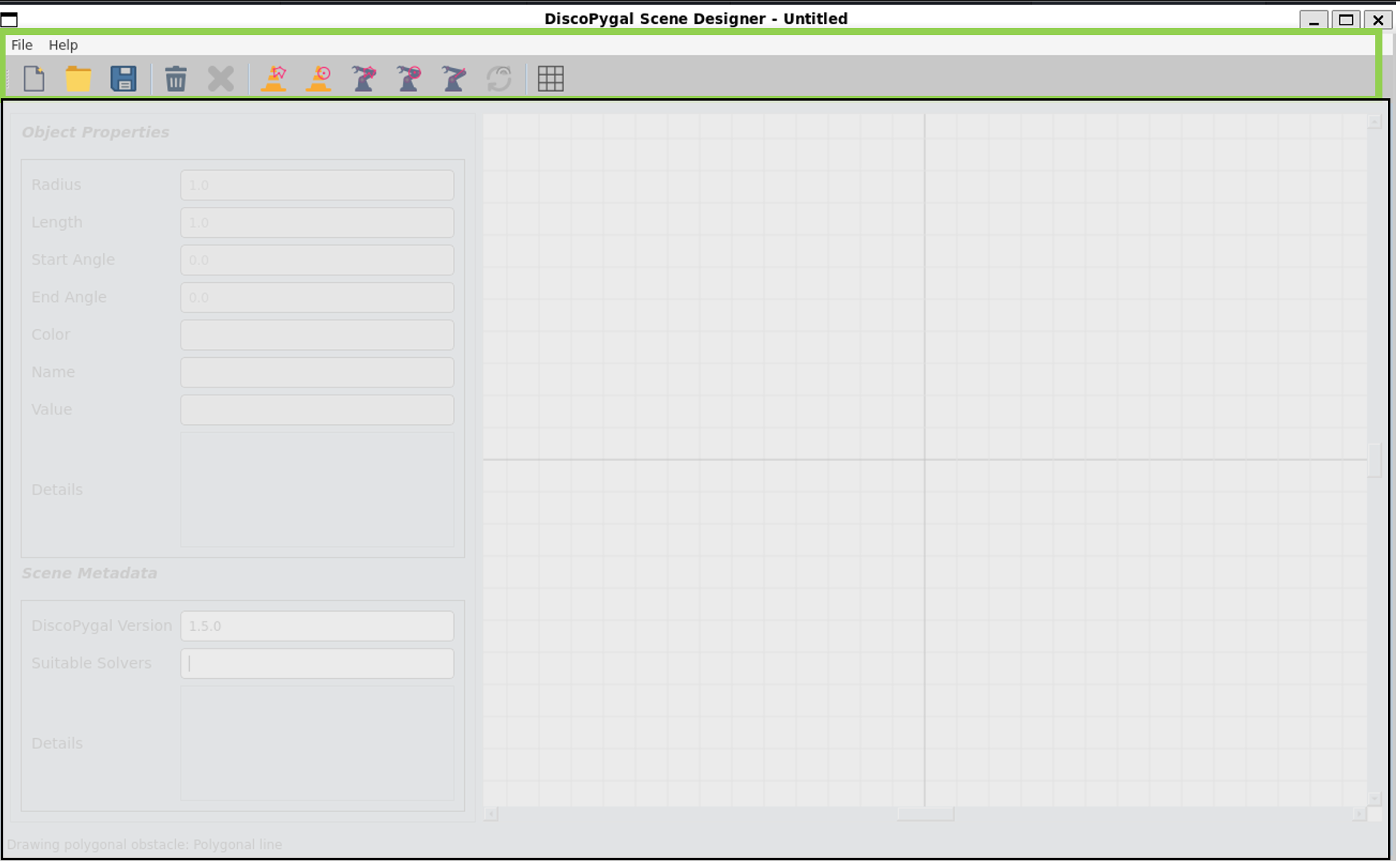
Toolbar / menu bar¶

The toolbar and menu bar provide access to all the main actions and drawing modes.

Icon	Action	What it does
	New (File → New)	Discard the current scene and start fresh. Prompts to save if there are unsaved changes.
	Open (File → Open)	Load a previously saved `.json` scene file.
	Save (File → Save)	Save to the current file path. Prompts for a path if the scene has never been saved.
	Save As (File → Save As)	Always prompts for a new file path.
	Quit (File → Quit)	Exit the application.
	Polygon obstacle	Switch drawing mode to polygon obstacle.
	Disc obstacle	Switch drawing mode to disc obstacle.
	Polygon robot	Switch drawing mode to polygon robot.
	Disc robot	Switch drawing mode to disc robot.
	Rod robot	Switch drawing mode to rod robot.
	Grid (View → Grid)	Toggle the background grid on/off.
	Randomize colors	Assign random HSV colors to all robots (or only the selected robot if one is selected).
	Clear scene	Remove all objects from the scene.
	Delete	Delete the currently selected object.
	Preferences	Open the preferences dialog.
	About	Show version and credits.

Canvas (viewport)¶

The large central area is the interactive canvas.

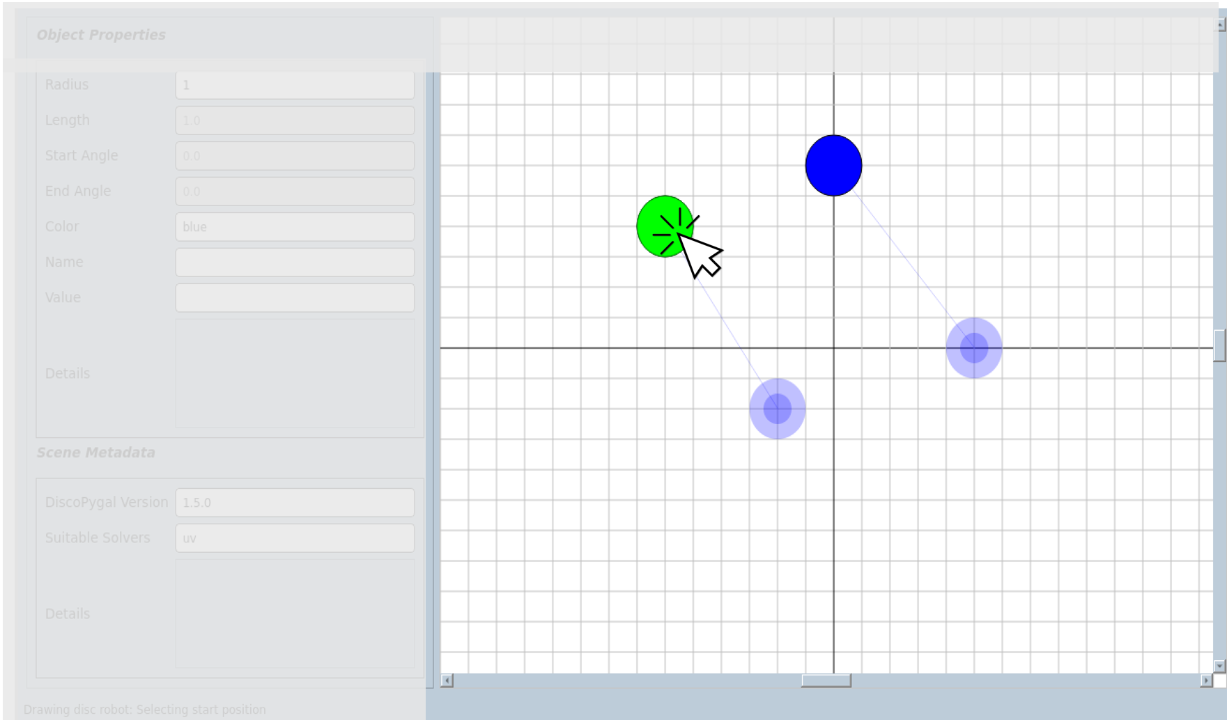
../_images/scene_designer_select_object.png

Left-click on an existing object to select it. Its properties appear in the Properties panel on the right.

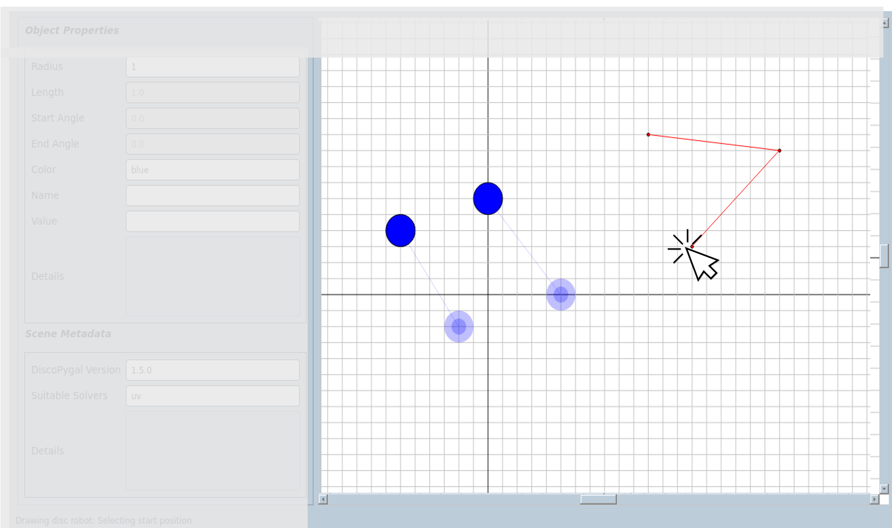
../_images/scene_designer_add_polygon.png

Right-click anywhere on the canvas while in a drawing mode to place a point (polygon vertex) or place a center (disc / rod).
Scroll / zoom controls follow the same conventions as the base GUI (use mousewheel to zoom).

Keyboard shortcuts¶

Shortcut	Action
`Delete`	Delete the currently selected object.
`Ctrl+z`	Undo the last action (where supported).
`Ctrl+y`	Redo the last undo action (where supported).
`Escape`	Cancel the current drawing operation.

Properties panel¶

The panel on the right-hand side shows and lets you edit the properties of the currently selected object. Fields are enabled or disabled automatically depending on the object type.

Geometry fields (enabled by object type)

Field	Applies to
`radius`	Disc obstacle, Disc robot
`length`	Rod robot
`start` `angle`	Rod robot (start angle in radians)
`end` `angle`	Rod robot (end angle in radians)

Metadata fields (enabled for any selected object)

Field	Meaning
`color`	Display color of the object. Accepts HSV strings in the format `HSV h,s,v` (e.g. `HSV 120,200,230`) or any color format recognised by Qt. Use Randomize colors from the toolbar to generate a valid HSV value.
`name`	A human-readable identifier for the object.
`value`	An arbitrary string value attached to the object; solvers may read this via `robot.data['value']`.
`details`	A multi-line free-text field for any extra notes about the object.

All metadata edits take effect immediately and mark the scene as changed (* in the title bar).

Scene metadata panel¶

Below or beside the Properties panel you will find fields that belong to the whole scene rather than to any single object:

Field	Meaning
`version`	The DiscoPygal version that created/last saved the scene. Read-only; updated automatically on save.
`solvers`	Free-text. Conventionally a comma-separated list of solver class names recommended for this scene.
`scene details`	Multi-line free-text description of the scene.

Step 4: Draw Objects¶

Drawing a polygon (obstacle or robot)¶

Select Polygon obstacle or Polygon robot from the toolbar.
Right-click on the canvas to place each vertex.
Close the polygon by clicking back on the first vertex (or using the designated close action for your version).
The finished polygon appears in the scene.

Drawing a disc (obstacle or robot)¶

Select Disc obstacle or Disc robot from the toolbar.
Right-click once on the canvas to place the center.
The disc appears with the default radius.
Left-click the disc to select it, then edit the radius field in the Properties panel.

Drawing a rod robot¶

Select Rod robot from the toolbar.
Right-click once on the canvas to place the rod’s reference point.
The rod appears with default length, start angle, and end angle values.
Left-click the rod to select it, then edit those fields in the Properties panel as needed.

Default geometry values¶

When you first draw an object, the geometry fields are filled with default values. You can read the current defaults from the constants OBJDRW_DEFAULT_RADIUS, OBJDRW_DEFAULT_LENGTH, OBJDRW_DEFAULT_START_ANGLE, and OBJDRW_DEFAULT_END_ANGLE in the object_drawer module.

Step 5: Select and Edit Objects¶

Selecting an object¶

Left-click any object on the canvas. A selection indicator appears and the Properties panel populates with that object’s current values.

Editing properties¶

With an object selected, simply type into the Properties panel fields. Every keystroke is applied immediately:

Geometry fields update the shape in real time.
Metadata fields (color, name, value, details) are stored in the object’s data dictionary and saved to JSON.

Deselecting¶

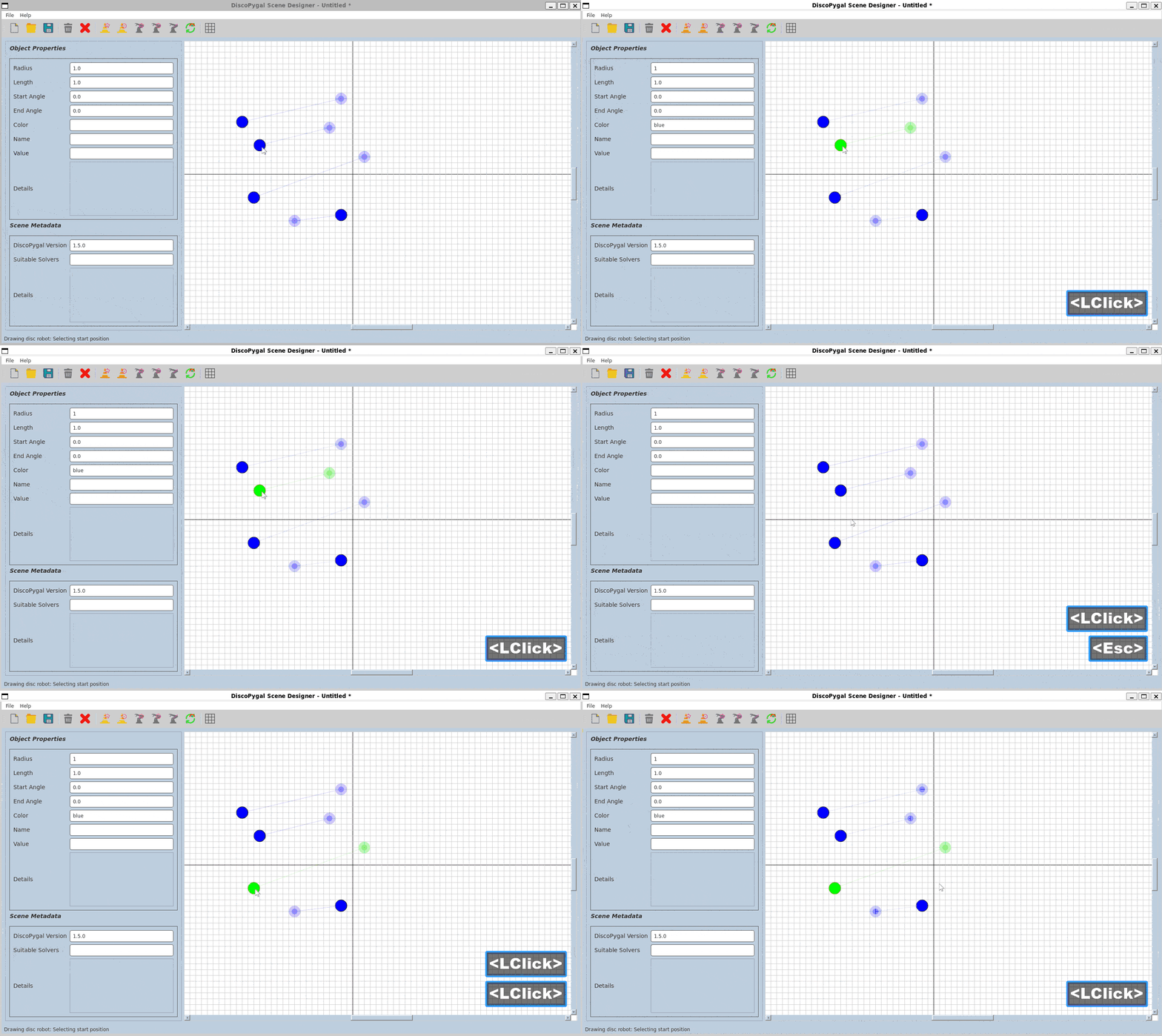
Left-click on empty canvas space, or press Escape to cancel any ongoing drawing operation (this also deselects).

Deleting an object¶

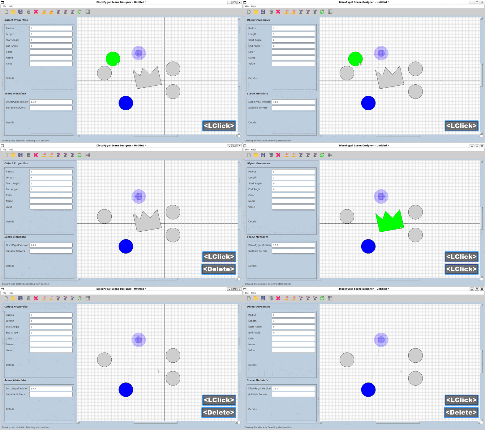
Select the object and press Delete, or use Edit → Delete from the menu. This removes the object from the scene immediately. The scene is marked as changed.

Step 6: Work with Colors¶

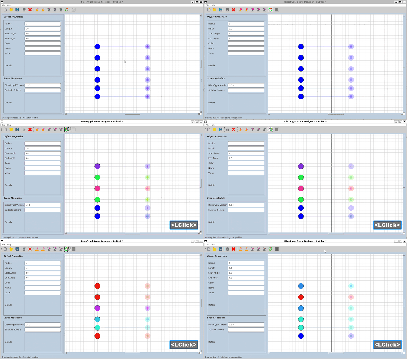
Every robot (and obstacle) can carry a color metadata value that controls how it is rendered. Colors are stored as strings in Qt-compatible formats, with HSV being the recommended format:

HSV <hue>,<saturation>,<value>
# Example: HSV 240,200,230  →  a medium blue

The Randomize colors toolbar action sets a random HSV color:

If a robot is currently selected, only that robot’s color is randomized.
If nothing is selected, all robots in the scene receive new random colors.

This is the fastest way to assign distinct colors when building multi-robot scenes.

Step 7: Use the Grid¶

The background grid helps with spatial alignment.

Toggle it on/off with View → Grid (or the Grid toolbar button).
Grid options (spacing, color, etc.) are accessible through the Preferences dialog (Edit → Preferences).

The grid state is a UI preference and is not saved to the scene JSON.

Step 8: Save and Load Scenes¶

Saving¶

Use File → Save (Ctrl+S in most builds) or File → Save As to write the scene to a .json file. The format is DiscoPygal’s standard scene dictionary produced by Scene.to_dict().

The title bar clears the * marker and updates to show the saved filename.

Loading¶

Use File → Open to open an existing scene. If there are unsaved changes in the current scene, a dialog asks whether to save, discard, or cancel.

After loading:

The scene version stored in the file is compared with the installed version. If they differ, the scene is marked as changed immediately so you are prompted to re-save with the current version.
All metadata fields in the UI (solvers, scene details) are repopulated from the file.

Starting fresh¶

File → New discards the current scene (after the same save-or-discard prompt) and resets everything to a blank scene with the current version stamp.

Unsaved-changes prompt¶

Whenever an action would discard unsaved work (New, Open, or Quit), a dialog offers three choices:

Save – save now, then continue.
Discard – throw away changes and continue.
Cancel – abort the action and return to the scene.

Step 9: Build a Complete Solvable Scene¶

Follow these steps to produce a scene that a solver can immediately use.

Launch the Scene Designer (Step 1: Launch the Scene Designer).
Add a boundary (optional but recommended): draw a large polygon obstacle that forms the outer walls of the workspace.
Add internal obstacles: switch to Polygon obstacle or Disc obstacle and draw the obstacles the robots must navigate around.
Add a robot: switch to Disc robot (simplest to start with) and right-click to place it. Select it and set a radius appropriate for your workspace.
Set start and goal: the scene format records start and goal as positional data on the robot object. Consult the solver documentation for the exact field names (typically stored via the name / value / details metadata fields or via dedicated start/goal position widgets, depending on your build).
Assign a color to the robot (use Randomize colors or type an HSV value directly).
Fill in scene metadata: in the solvers field, enter the name of the solver you intend to use. Add a human-readable note in scene details.
Save the scene (File → Save) to a .json file, for example my_first_scene.json.

Step 10: Understanding Scene Serialization and JSON Format¶

When you save a scene using the Scene Designer, it is stored as a JSON file. Understanding this format is useful for debugging, sharing scenes, or programmatically working with them.

JSON Structure Overview¶

A DiscoPygal scene JSON file has this top-level structure:

{
    "__class__": "Scene",
    "obstacles": [...],
    "robots": [...],
    "metadata": {...}
}

The __class__ field identifies the object type for deserialization.

Obstacles in JSON¶

Obstacles are stored in the "obstacles" array. There are two types:

Disc Obstacle:

{
    "__class__": "ObstacleDisc",
    "location": [x, y],
    "radius": 5.0,
    "data": {
        "color": "HSV 180,200,230",
        "name": "obstacle_1"
    }
}

Polygon Obstacle:

{
    "__class__": "ObstaclePolygon",
    "poly": [[x1, y1], [x2, y2], [x3, y3], ...],
    "data": {
        "color": "HSV 180,200,230",
        "name": "wall"
    }
}

Robots in JSON¶

Robots are stored in the "robots" array. There are three types:

Disc Robot:

{
    "__class__": "RobotDisc",
    "radius": 2.5,
    "start": [x_start, y_start],
    "end": [x_goal, y_goal],
    "data": {
        "color": "HSV 0,200,230",
        "name": "robot_1"
    }
}

Rod Robot:

{
    "__class__": "RobotRod",
    "length": 10.0,
    "start": [[x_start, y_start], angle_start],
    "end": [[x_goal, y_goal], angle_goal],
    "data": {
        "color": "HSV 120,200,230",
        "name": "rod_robot"
    }
}

Polygon Robot:

{
    "__class__": "RobotPolygon",
    "poly": [[x1, y1], [x2, y2], ...],
    "start": [x_start, y_start],
    "end": [x_goal, y_goal],
    "data": {
        "color": "HSV 240,200,230",
        "name": "polygon_robot"
    }
}

Scene Metadata¶

The "metadata" field stores scene-level information:

"metadata": {
    "version": "0.5.0",
    "solvers": "DiscRRTStar, TaucGL",
    "scene_details": "A narrow corridor scenario for testing navigation"
}

The version field is auto-populated with the DiscoPygal version when the scene is saved.

Loading and Working with Scenes Programmatically¶

You can work with scene JSON files in Python using the Scene class:

from discopygal.solvers_infra import Scene

# Load a scene from a JSON file
scene = Scene.from_file('my_scene.json')

# Access robots and obstacles
for robot in scene.robots:
    print(f"Robot at {robot.start}, heading to {robot.end}")

# Modify and save
scene.add_robot(new_robot)
modified_dict = scene.to_dict()

# Save back to JSON
import json
with open('modified_scene.json', 'w') as f:
    json.dump(modified_dict, f, indent=2)

Key Conversion Functions:

All coordinates in JSON are floats (not CGAL types). The serialization process uses conversion functions:

Point_2 ↔ [x, y] coordinate pairs
FT (field type) ↔ float values
Polygons ↔ arrays of coordinate pairs

The load_object_from_dict() function automatically handles reconstruction of the correct object type based on the __class__ field.