Introduction to CGALPY
In this tutorial, we will show the basic concepts of CGALPY and how to use it. Note that this is not a comprehensive documentation of all available features, but we do try to include the most useful (in our opinion) capabilities and examples.
CGALPY is a Python port of CGAL, which was originally written in C++. The port was made using the power of boost::python. The Computational Geometry Algorithms Library (CGAL) is a suite of computational geometry algorithms, which is used by many professionals and academies around the world. It provides advanced algorithms with excellent performance, while also addressing edge cases and various issues of robustness.
All of the code snippets in this tutorial which are more than a few lines are self contained, and should run as is (without any modifications).
Basic Concepts
Before tackling the more algorithmic/complex structures and ideas of CGAL (and CGALPY), we will explain briefly what a kernel is, and a few core entities which one must know to use CGALPY properly.
CGALPY.Ker
A kernel is a collection of geometric primitive objects, and operations on these objects. Different kernels have different capabilities, and each has its tradeoffs. Note that the default installation of CGALPY has a predetermined kernel which has the broadest appeal (having the most exact constructions/results, but has a drop in performance in some cases) - hence you should not be too bothered in which kernel to use, but what primitives does it have. The kernel can be accessed by:
import CGALPY

Ker = CGALPY.Ker # Ker is the module containing all the kernel objects
CGALPY.Ker.FT
Represents a single, real number. FT is a an abbreviation for “Field Type”, and different kernels have different types - but you can think about it as an alternative to Python’s float. Any other CGAL object expects to get numbers in the FT format (and not Python floats). Below is an example of how to convert between FT and float:
import CGALPY

# CGALPY Modules and objects
Ker = CGALPY.Ker
FT = Ker.FT

# Convert from python float to FT
x = FT(1.24)
print(x)

# Convert from FT to float
y = x.to_double()
print(y)

# You can also do arithmetic with FTs
z = (FT(1.24) + FT(2.0)) / FT(3.0)
print(z)
CGALPY.Ker.Point_2
Represents a 2D point, with x and y coordinates. Note that x and y values are of type FT!
import CGALPY

# CGALPY Modules and objects
Ker = CGALPY.Ker
FT = Ker.FT
Point_2 = Ker.Point_2

# Generate a 2D point
p = Point_2(FT(1.24), FT(2.0))
print(p)

# Access x and y values (both are of type FT)
x = p.x()
y = p.y()
print(x, y)
CGALPY.Ker.Segment_2
Represents a linear segment connecting two 2D points. The linear segment is directed - where the first point is the starting point, and the second is the ending point.
import CGALPY

# CGALPY Modules and objects
Ker = CGALPY.Ker
FT = Ker.FT
Point_2 = Ker.Point_2
Segment_2 = Ker.Segment_2

# Generate a segment
p = Point_2(FT(1.24), FT(2.0))
q = Point_2(FT(0.0), FT(0.0))
segment = Segment_2(p, q)
print(segment)

# Access source and target points (both are of type Point_2)
s = segment.source()
t = segment.target()
print(s, t)
CGALPY.Ker.Circle_2
Represents a circle with a center point (as a Point_2) and a squared radius (as FT) - i.e.  . A circle is also directed - it can be clockwise or counter-clockwise.
The radius is squared since for most geometric purposes, it allows for much more exact constructions (and hence results).
import CGALPY

# CGALPY Modules and objects
Ker = CGALPY.Ker
FT = Ker.FT
Point_2 = Ker.Point_2
Circle_2 = Ker.Circle_2

# Generate a segment (clockwise and counter-clockwise)
center = Point_2(FT(1.0), FT(2.0))
radius = FT(1.24)
cw_circle = Circle_2(center, radius * radius, Ker.CLOCKWISE)
ccw_circle = Circle_2(center, radius * radius, Ker.COUNTERCLOCKWISE)
print(cw_circle)
print(ccw_circle)

# Access center and (squared) radius
cw_center = cw_circle.center()
cw_squared_radius = cw_circle.squared_radius()
print(cw_center, cw_squared_radius)
CGALPY.Ker.Vector_2
Similar to Point_2, but represents a direction (vector) instead of a 2D point. You can add a vector to a point to transform it.
import CGALPY

# CGALPY Modules and objects
Ker = CGALPY.Ker
FT = Ker.FT
Point_2 = Ker.Point_2
Vector_2 = Ker.Vector_2

# Generate a vector
v = Vector_2(FT(1.0), FT(1.0))
print(v)

# Transform a Point_2
p = Point_2(FT(2.0), FT(3.0))
q = p + v
r = p - v
print(p, q, r)

# You can also do vector arithmetic
v1 = Vector_2(FT(1.0), FT(1.0))
v2 = Vector_2(FT(2.0), FT(3.0))
v3 = v2 - v1
print(v1, v2, v3)
2D Arrangements
This section was adapted from the 2D Arrangements manual in CGAL’s original documentation: https://doc.cgal.org/latest/Arrangement_on_surface_2/index.html#Chapter_2D_Arrangements Some details are omitted here for simplicity. You can visit the manual for more advanced capabilities and explanations.
A core concept in computational geometry is the arrangement. Given a set of curves  , the arrangement
  is the subdivision of the space
into zero, one and two-dimensional cells. These cells are called (respectively) the vertices, edges and faces induced by .
To clarify, a curve might be a linear segment, a circle or a circle segment (part of a circle). The curves can also intersect each other, and each intersection induces a new vertex in the arrangement.
is the subdivision of the space
into zero, one and two-dimensional cells. These cells are called (respectively) the vertices, edges and faces induced by .
To clarify, a curve might be a linear segment, a circle or a circle segment (part of a circle). The curves can also intersect each other, and each intersection induces a new vertex in the arrangement.
This structure can be described using a doubly-connected edge list data structure (DCEL), which contains the vertices, edges and faces plus the incidence relations among these cells. The main idea is to split each edge to two “halfedges” - one for each direction. After doing that - we ensure that for each halfedge we have consistency for a “source” and “target” vertices, as well as the notion of “incident face” is well defines - define it as the face that lies to the right of the halfedge.
Below is an example for a DCEL:

The arrangements module can be accessed as follows:
import CGALPY

Aos2 = CGALPY.Aos2 # Aos2 is the 2D arrangements module
Generating a simple arrangement
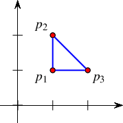
We will generate the following arrangement, containing two faces - the triangle  and the unbounded face (which will be generated implicitly).
Note that when inserting segments/curves to the arrangement, they should be of type Curve_2 under the traits submodule of the arrangement. When inserting a point into the arrangement, it should be of type TPoint under the traits submodule of the arrangement. Both Curve_2 and TPoint has an exact interface as their kernel counterparts. Conversion is straightforward:
# CGALPY Modules and objects
# ...
Aos2 = CGALPY.Aos2
Curve_2 = Aos2.Traits.Curve_2
TPoint = Aos2.Traits.Point_2
# ...

# Convert from Segment_2 to Curve_2
segment = Segment_2(...)
curve = Curve_2(segment)

# Convert a Point_2 to TPoint
point = Point_2(...)
tpoint = TPoint(point.x(), point.y())
We will also print the number of vertices, edges and faces in the arrangement.
import CGALPY

# CGALPY Modules and objects
Ker = CGALPY.Ker
FT = Ker.FT
Point_2 = Ker.Point_2
Segment_2 = Ker.Segment_2

Aos2 = CGALPY.Aos2
Arrangement_2 = Aos2.Arrangement_2
Curve_2 = Aos2.Traits.Curve_2
TPoint = Aos2.Traits.Point_2

# Create the points and segments
p1 = Point_2(FT(1), FT(1))
p2 = Point_2(FT(1), FT(2))
p3 = Point_2(FT(2), FT(1))
segments = [Segment_2(p1, p2), Segment_2(p2, p3), Segment_2(p3, p1)]

# Generate an empty arrangement and insert the segments
arr = Arrangement_2()
Aos2.insert(arr, [Curve_2(segment) for segment in segments]) # Note that we convert Segment_2 to Curve_2

# Insert an isolated vertex
q = Point_2(FT(0), FT(0))
Aos2.insert_point(arr, TPoint(q.x(), q.y()))

# Print the number of vertices, edges and faces
print(arr.number_of_vertices())
print(arr.number_of_edges())
print(arr.number_of_faces())
Traversing the Arrangement
The simplest and most fundamental arrangement operations are the various traversal methods, which allow users to systematically go over the relevant features of the arrangement at hand.
First we note that the arrangement gives rise to three new object types, which are the handles - references to an object (vertex/halfedge/face) in the arrangement. These types can be accessed as follows:
import CGALPY

Aos2 = CGALPY.Aos2
Arrangement_2 = Aos2.Arrangement_2
Face = Arrangement_2.Face
Halfedge = Arrangement_2.Halfedge
Vertex = Arrangement_2.Vertex
First we note that you can traverse all objects (without any meaningful order):
import CGALPY

# CGALPY Modules and objects
Ker = CGALPY.Ker
FT = Ker.FT
Point_2 = Ker.Point_2
Segment_2 = Ker.Segment_2

Aos2 = CGALPY.Aos2
Arrangement_2 = Aos2.Arrangement_2
Curve_2 = Aos2.Traits.Curve_2

# Create the points and segments
p1 = Point_2(FT(1), FT(1))
p2 = Point_2(FT(1), FT(2))
p3 = Point_2(FT(2), FT(1))
segments = [Segment_2(p1, p2), Segment_2(p2, p3), Segment_2(p3, p1)]

# Generate an empty arrangement and insert the segments
arr = Arrangement_2()
Aos2.insert(arr, [Curve_2(segment) for segment in segments]) # Note that we convert Segment_2 to Curve_2

# Traverse the arrangement
for vertex in arr.vertices():
    print(vertex)
for halfedge in arr.edges(): # For every edge, this returns only *one* halfedge
    print(halfedge)
for halfedge in arr.halfedges(): # For every edge, returns both halfedges
    print(halfedge)
for face in arr.faces():
    print(face)
Note that all the methods above (vertices(), edges(), halfedges(), faces()) are iterators. Also note again that the order of objects has no meaningful meaning, and subscripting objects (i.e. vertices[i]) is unreliable for the DCEL data structure.
Traversal Methods for an Arrangement Vertex
Assume we have a vertex handle (for example take the first vertex from the arr.vertices() iterator):
vertex = next(arr.vertices())
To access the underlying TPoint of the vertex:
vertex.point() # Returns TPoint
To check if the vertex is isolated (i.e. has no incident halfedge):
vertex.is_isolated() # Return True if isolated
To traverse all incident halfedges (halfedges for which the given vertex is the target):
for halfedge in vertex.incident_halfedges():
    print(halfedge)
To get the degree of the vertex (number of incident halfedges):
vertex.degree() # Returns int
If the vertex is isolated, we can obtain the face that contains it:
assert(vertex.is_isolated) # Make sure the vertex is isolated
vertex.face() # Returns Face
Traversal Methods for an Arrangement Halfedge
Assume we have a halfedge handle (for example take the first halfedge from the arr.edges() iterator):
halfedge = next(arr.edges())
We can get the underlying curve, as well as the source and target vertices:
halfedge.curve() # Returns X_monotone_curve_2 which is similar to Curve_2
halfedge.source() # Returns Vertex
halfedge.target() # Returns Vertex
To get the twin halfedge (the same edge but in reverse direction):
halfedge.twin() # Returns Halfedge
And by the definition of the twin we get the following:
assert(halfedge.curve() == halfedge.twin().curve())
assert(halfedge.source() == halfedge.twin().target())
assert(halfedge.target() == halfedge.twin().source())
To get the incident face of a halfedge (the face that lies to its left):
halfedge.face() # Returns Face
Note that a halfedge is always one link in a connected chain “boundary” (CCB) of halfedges that share the same incident face (i.e. a boundary of that incident face). To get the next and previous halfedges in the CCB:
halfedge.next() # Returns Halfedge
halfedge.prev() # Returns Halfedge
We can also iterate over all the edges in the CCB:
for curr in halfedge.ccb():
    print(curr.source().point(), curr.target().point()) # type(curr) is Halfedge
Traversal Methods for an Arrangement Face
Assume we have a face handle (for example take the first face from the arr.faces() iterator):
face = next(arr.faces())
Recall that the arrangement has one unbounded face. We can check if a given face is unbounded:
face.is_unbounded() # Returns bool
We can also get directly the unbounded face of the arrangement:
arr.unbounded_face() # Returns Face
Any bounded face has an outer boundary (or outer CCB), which we can iterate. Note that the halfedges along this CCB wind in a counterclockwise order around the outer boundary of the face.
for halfedge in face.outer_ccb():
    print(halfedge)
A face can also contain disconnected components in its interior, namely, holes and isolated vertices. You can access these components as follows:
# To access holes:
num_of_holes = face.number_of_inner_ccbs() # Returns int
for hole in face.holes():
    for halfedge in hole:
        print(halfedge)

# To access isolated vertices:
num_if_isolated_verts = face.number_of_isolated_vertices()
for vertex in face.isolated_vertices():
    print(vertex.point())
Point Location Queries
Given a point, we would like to find in which object of the arrangement it is contained (it might be a face, halfedge or even coinciding with an existing vertex).
There are many strategies for point-location algorithms, but in this tutorial we will use the trapezoid RIC strategy, but all strategies can be interchanged with minimal to no changes. To read about the different strategies and their advantages (or disadvantages) please refer to the original manual.
In order to use a point location algorithm, we need to construct an ArrangementPointLocation_2 object - which will run some preprocessing on the arrangement. We can then use that object to query points on the arrangement.
import CGALPY

# ...
Arr_trapezoid_ric_point_location = Aos2.Arr_trapezoid_ric_point_location

# Point location is done with TPoint (and not Point_2)
arr = Arrangement_2()
# ... insert curves to the arrangement
point_location = Arr_trapezoid_ric_point_location(arr)

query = Point_2(...)
query = TPoint(query.x(), query.y())

obj = point_location.locate(query) # Obj is now a point location result

v = Vertex()
he = Halfedge()
f = Face()

if obj.get_vertex(v):
    # if obj is a vertex, then v will now have the query result
    # ...
elif obj.get_halfedge(he):
    # if obj is a halfedge, then he will now have the query result
    # ...
elif obj.get_face(f):
    # if obj is a face, then f will now have the query result
    # ...
The following example will construct the triangle above, and then query four points - two that lie in the interior of a face (the face of the triangle and the unbounded face), one that lies on an edge and one the coincides with a vertex.
import CGALPY

# CGALPY Modules and objects
Ker = CGALPY.Ker
FT = Ker.FT
Point_2 = Ker.Point_2
Segment_2 = Ker.Segment_2

Aos2 = CGALPY.Aos2
Arrangement_2 = Aos2.Arrangement_2
Curve_2 = Aos2.Traits.Curve_2
TPoint = Aos2.Traits.Point_2

Vertex = Arrangement_2.Vertex
Halfedge = Arrangement_2.Halfedge
Face = Arrangement_2.Face

Arr_trapezoid_ric_point_location = Aos2.Arr_trapezoid_ric_point_location


# Create the points and segments
p1 = Point_2(FT(1), FT(1))
p2 = Point_2(FT(1), FT(2))
p3 = Point_2(FT(2), FT(1))
segments = [Segment_2(p1, p2), Segment_2(p2, p3), Segment_2(p3, p1)]

# Generate an empty arrangement and insert the segments
arr = Arrangement_2()
Aos2.insert(arr, [Curve_2(segment) for segment in segments]) # Note that we convert Segment_2 to Curve_2
point_location = Arr_trapezoid_ric_point_location(arr)

queries = [
    Point_2(FT(1.25), FT(1.25)), # Lies inside the triangle
    Point_2(FT(0), FT(0)), # Lies outside the triangle
    Point_2(FT(1.5), FT(1)), # Lies on a halfedge
    Point_2(FT(1), FT(1)), # Coincides with a vertex
]

for query in queries:
    print('\n', query)
    query = TPoint(query.x(), query.y()) # Convert to TPoint
    v = Vertex()
    he = Halfedge()
    f = Face()

    obj = point_location.locate(query)

    if obj.get_vertex(v):
        print('Coincides with vertex:')
        print('\t', v.point())
    elif obj.get_halfedge(he):
        print('Lies on a halfedge:')
        print('\t', he.source().point(), he.target().point())
    elif obj.get_face(f):
        print('Lies in a face interior:')
        if f.is_unbounded():
            print('\tOutside the triangle')
        else:
            print('\tInside the triangle')
Intersecting with Curves
In a similar fashion to point location, if we would like to find all arrangement objects that intersect with a given curve, we can use the zone() function:
arr = Arrangement_2(...)
point_location = Arr_trapezoid_ric_point_location(arr)

res = []
curve = Curve_2(...)
Aos2.zone(arr, curve, res, point_location) # res will now have all intersecting objects

for obj in res:
    if type(obj) is Vertex:
        # ...
    elif type(obj) is Halfedge:
        # ...
    elif type(obj) is Face:
        # ...
Removing Vertices and Edges
The function remove_vertex can only remove isolated or redundant vertices (i.e. vertices that have exactly two incident edges which can be merged into a single curve). If it is neither the function will return an indication that it has failed to remove the vertex.
Aos2.remove_vertex(arr, vertex)
The function remove_edge removes an edge from the arrangement, and if either of the end vertices becomes isolated or redundant after the removal of the edge, it removes the vertex as well.
Aos2.remove_edge(arr, halfedge)
Face Data and Map Overlay
One useful application of arrangements is the ability to perform map overlays quite easily. Map overlay is the arrangement generated by the union of the curves of the underlying arrangements.
For example, assume that we are given two geographic maps represented as arrangements, with some data objects attached to their faces, representing some geographic information - for instance, a map of the annual precipitation in some country and a map of the vegetation in the same country - and you are asked to locate, for example, places where there is a pine forest and the annual precipitation is between 1,000 mm and 1,500mm. Overlaying the two maps may help you figure out the answer.
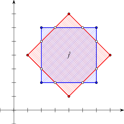
Before we show how to overlay two arrangements, we note that for many cases it can be useful to first attach some data to the faces of the arrangement. Doing that, we can also describe to the overlay algorithm what to do when two faces of the arrangements overlap (like in the image above - the overlapping area is colored in purple).
To add a data to a face:
face.set_data(data) # data is a Python object
To get a face data:
face.data()
Now to overlay two arrangements, we need to define “overlay traits” - which in our case tell the overlay algorithm what to do in case of overlapping faces. Note that traits is a fairly advanced concept in the architecture of CGAL, which we will not describe here (but it is described in detail in the CGAL manual).
import CGALPY

# ...
Arr_overlay_function_traits = Aos2.Arr_overlay_function_traits

# Define the overlay traits, which get a function of (x, y) where
# x, y are the data objects of the faces and it returns the data of the overlapped face.
# If for example, the data is an integer - for overlapping areas we can just sum
traits = Arr_overlay_function_traits(lambda x, y: x + y)

# Now we can overlay arr1 and arr2, and store the result in arr
arr1 = Arrangement_2(...)
arr2 = Arrangement_2(...)
arr = Arrangement_2(...)

Aos2.overlay(arr1, arr2, arr, traits)