Boolean Network Model

According to this model the network is represented as an oriented graph G = (V, F), whose nodes V represent element of the network, and F defines a topology of edges between the nodes and a set of boolean functions. A node may represent either a gene or a biological stimulus, where a stimulus is any relevant physical or chemical factor which influences the network and is itself not a gene or gene product. A node has an associated steady-state expression level x_v , representing the amount of gene product (in the case of a gene) or the amount of stimulus present in the cell. This level is approximated as high or low and represented by the binary value 1 or 0, respectively. Network behavior over time is modelled as a sequence of discrete synchronous steps. The set $F= {\{f_v \vert v \in V\}}$ of boolean functions assigned to the nodes defines the value of a node on the next step depending on values of other nodes, which influence it. The functions f_v are uniquely defined using truth tables. An edge directed from one node to another represents the influence of the first gene or stimulus on that of the second, so that the expression level of a node v is a Boolean function f_v of the levels of the nodes in the network which connect (have a directed edge) to v. We sometimes confuse the network with its undirected underlying graph G(V,E). 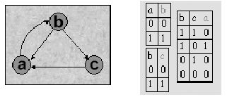The following figures 14.6 give an example of a simple boolean network and associated truth tables. This example shows a network of three nodes - a, b and c. As one can see, expression of c directly depends on expression of b, which directly depends on a. However, influence of b and c on a is more complex. For example, high level of expression of both b and c leads to inhibition of a.

  

Figure: Sample boolean network - adapted from [8]

The assignment of values to nodes fully describes the state of the model at any given time. The change of model state over time is fully defined by the functions in F. Initial assignment of values uniquely defines the model state at the next step, and, consequently, on all the future steps. Thus, the network evolution is realized as a sequence of consecutive states, and it is uniquely defined by the initial state. Such a sequence of states is called trajectory. 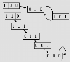Figure 14.7 shows two such trajectories for our sample network. Since the number of possible states is finite, all trajectories eventually end up in single steady state, or a cycle of steady states.

  

Figure: States trajectories - adapted from [8]

• An attractor of a trajectory is a single steady state, or a cycle at the end of the trajectory.
• The basin of attraction for a specific attractor is a set of all trajectories leading to it.

The network in our example has two attractors - one is the steady state (0,0,0), and the other is a cycle $(0,1,0) \leftrightarrow (1,0,1)$. States in gene networks are often characterized by stability - "slight" changes in value of a few nodes do not change the attractor. Biological systems are often redundant to ensure that the system stays stable and retains its function even in presence of local anomalies. For example, there may be two proteins, or even two different networks with the same function, which backup each other.