Computing the Likelihood of a Tree

For the analysis below, we shall use the following terms:

 

. A reconstruction is a full labeling of the tree's internal nodes. A branch length t_vu is the length of the edge between nodes v and u, and it measures the biological time, or genetic distance, between the species associated with these nodes. As always, we assume that the characters are pairwise independent, and that the branching is a Markov process, that is, the probability of a node having a given label is a function only of the state of the parent node and the branch length, t, between them. Our model also includes a distance function to compute the latter probability, i.e.: $P_{x \rightarrow y}(t_{vu})$, the probability that state x will transform into state y within the time t_vu. We further assume that the character frequencies are fixed throughout the evolutionary history, and that they are given as P(x).

Problem 9.11   Likelihood of a Tree.
INPUT:

• A matrix M describing a set of m characters for each one of n given species.
• A tree T with the above species as its leaves and with known branch lengths t_vu.

QUESTION: Calculate the likelihood L of the tree: L = P(M|T).

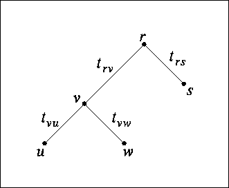
First, let us deal with a simple case, where there is only one character identifying each species. Since the labels of the internal nodes are unknown, we need to sum over all possible reconstructions. For example, for the tree illustrated in figure 9.10, we can immediately write down the following formula:

$$L = P(M\vert T) = \sum_{r} \sum_{v} P(r) \cdot P_{r \right... ..._{v \rightarrow u}(t_{vu}) \cdot P_{v \rightarrow w}(t_{vw})$$ (9.9)

where r and v are possible labels (character values) for the corresponding nodes.

  

Figure 9.10: A simple tree with branch lengths. The likelihood of this tree is calculated in equation 9.10.

To expand the formula for multiple characters, we simply need to repeat the above calculation for each character separately, and then multiply the results (recall the assumption that the characters are pairwise independent). The general equation is now:

$$P(M\vert T) = \prod_{\rm {character} \ j} P(M_j\vert T)$$ L =

$$\prod_{\rm {character} \ j} \ \{\ \sum_{\rm {reconstruction} \ R} P(M_j,R\vert T)\ \}$$ =

$$\prod_{\rm {character} \ j} \ \{\ \sum_{\rm {reconstruction} \ R}... ...t \prod_{\rm {edge} \ u \rightarrow v} P_{u \rightarrow v}(t_{uv})\ \rgroup\ \}$$ = (9.10)

Note: The trees inferred by maximum likelihood appear from this description to be rooted trees. However, if the model of character substitution is reversible, i.e., $P_{x \rightarrow y}(t) = P_{y \rightarrow x}(t)$, then the tree is actually unrooted - the root can be chosen arbitrarily, without any change in the likelihood of the tree. It now remains to show how this calculation can be performed efficiently. The following dynamic-programming ``pruning'' algorithm was introduced by Felsenstein  [3].

Calculating the likelihood of a tree using Dynamic Programming:
For a character j, denote:

$$C_j(x,v) = P (\mbox{\ subtree whose root is\ }v \ \vert\ v_j = x \ )$$

C_j(x,v) is the conditional likelihood of v's subtree, i.e., the probability of everything that is observed from node v on the tree down to the leaves, at character position j, given that v has the label x at this position.

• Initialization:
  For each leaf v and state x:
  

  $$C_j(x,v) = \left\{ \begin{array}{ll} 1 & v_j = x \\ 0 & \rm {otherwise} \end{array} \right.$$ (9.11)

  
  

• Recursion:
  Traverse the tree in postorder; for an internal node v with children u and w, compute for each possible state x:
  

  $$C_j(x,v) = \lgroup \ \sum_y C_j(y,u) \cdot P_{x \rightarrow y... ...p\ \sum_y C_j(y,w) \cdot P_{x \rightarrow y}(t_{vw})\ \rgroup$$ (9.12)

  
  

• The final solution is:
  

  $$L = \prod_{j=1}^{m} \ \lgroup \ \sum_x C_j(x,root) \cdot P(x)\ \rgroup$$ (9.13)

  
  

Complexity: For n species, m characters, and k possible states for each character, we perform $O(m \cdot k^2)$ work in O(n) nodes, so the running time of the algorithm is $O(n \cdot m \cdot k^2)$.