Molecular Surface Representation

Representing a protein by its molecular surface representation helps us in the study of protein folding [9], in prediction of biomolecular recognition, detection of drug binding 'cavities' and Molecular Graphics.

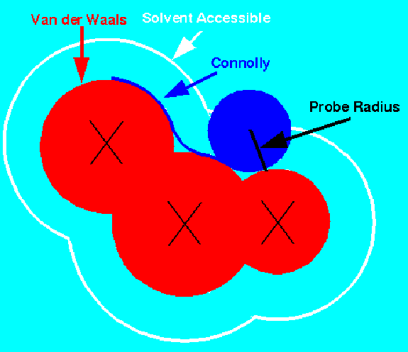
A common representation is due to Connolly [2]. It virtually rolls a 'water' probe ball (1.4-1.8 Å diameter) over the Van der Waals surface, smoothing the surface and bridging narrow crevices, which are inaccessible to the solvent. This partitions the surface into convex, concave and saddle patches according to the number of contact points between the surface atoms and the probe ball. As Output, the representation consists of points + normals to the surface. These are sampled according some required sampling density (e.g. 10 pts/Ų).

  

Figure 13.10: Connolly's Solvent Accessible Surface. Image taken from http://www.chem.leeds.ac.uk/ICAMS/eccc/cangaroo.html.

  

Figure 13.11: The molecular surface of Crambin is shown above, with the convex spherical patches colored yellow, the saddle-shaped pieces of tori colored green, and the concave reentrant surface colored blue. Image taken from http://www.netsci.org/Science/Compchem/feature14f.html.

There are different ways to represent shape complementarity. The points + normals representation [2] is a dense one. The points representation in [10] is sparser, and so is the Solid Angle local extrema [1]. Another representation is SPHGEN [5] - surface cavity modeling by pseudo-atom centers.

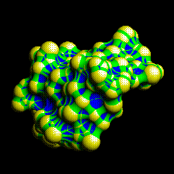
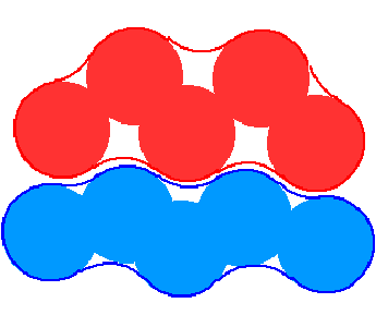
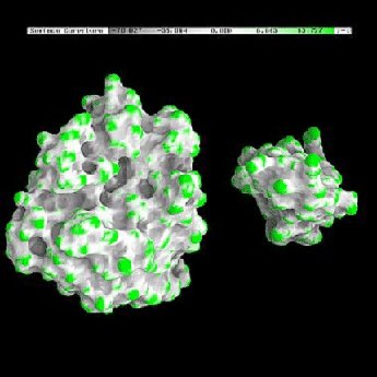
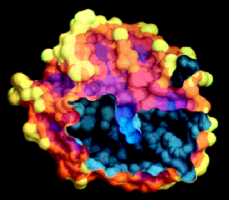
One of the advantages of the molecular surface is its ability to visualize the shape complementarity at interfaces, as show on figures 13.12 and 13.13.

  

Figure 13.12: Shape complementarity at interfaces. Taken from http://www.netsci.org/Science/Compchem/feature14e.html

  

Figure 13.13: Trypsin/Trypsin inhibitor. Figure from B. Honig's Labs web-site at Columbia University.

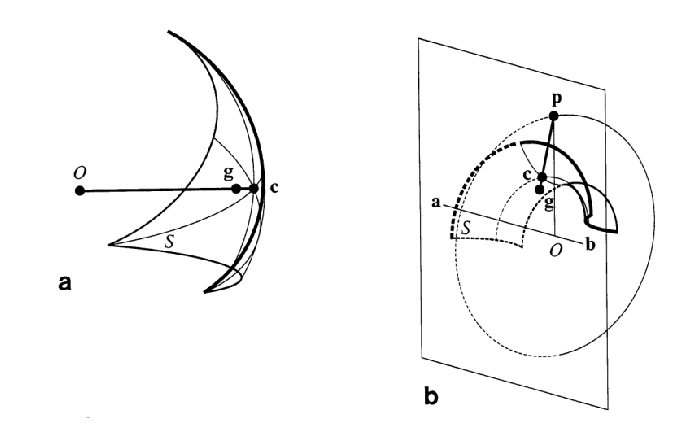
In the critical points representation based on Connolly's representation we define a single point and a normal for each patch, as illustrated in figure 13.14. Convex patches are called caps, concave ones - pits and saddles are called belts.

  

Figure 13.14: An illustration of the generation of (a) caps and pits, and (b) belts, respectively. Symbols are as follows: S is a Connolly face, either convex (for caps) or concave (for pits) (a), and saddle-shaped (for belts) (b); O in (a) is either the atomic center (for caps) or the probe center (for pits). In (b), O is the center of the torus central circle; in (a) and (b), g is the gravity center of a face and c is its projection on the surface. Also in (b): a and b are the two atoms along which the torus axis lies, and p is where the straight line throught c and g intersects the plain normal to ab, that passes through O.

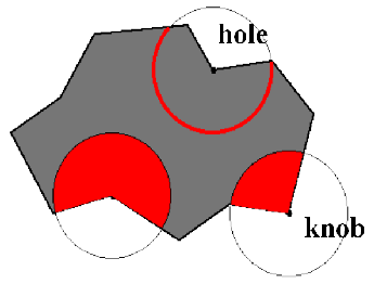
The Solid Angle local extrema (knobs - holes) representation is based upon centering a sphere at the protein surface and measuring the fraction of the sphere inside the solvent-excluded volume of the protein. If more than half of the sphere is inside the protein, the region is concave, if less than half of the sphere is inside the protein, the shape is convex. Either the solid sphere or the sphere surface may be used. A two-dimensional example is shown in figure 13.15.

  

Figure 13.15: Solid Angle local extrema. Taken from http://www.netsci.org/Science/Compchem/feature14h.html

  

Figure: The chymotrypsin surface above has been colored according to convexity or concavity. A sphere of radius 6 Å was centered at several points on each surface face, and the solid angle of the sphere lying inside the protein's molecular surface was computed and averaged over the face. Each face was colored according to where its average solid angle fell in the range between zero and four ${\pi }$ steradians. Convex regions are yellow, concave regions are blue, and regions of intermediate curvature are orange, red, and purple. The surface has been clipped, and the inner side of the molecular surface has been colored grey. The substrate-binding pocket is at the center of the image and can be seen to be blue. Taken from http://www.netsci.org/Science/Compchem/feature14h.html.

The SPHGEN representation generates sets of overlapping spheres to describe the shape of a molecule or molecular surface. For receptors, a negative image of the surface invaginations is created; for a ligand, the program creates a positive image of the entire molecule. Each sphere touches the molecular surface at two points and has its radius along the surface normal of one of the points. For the receptor, each sphere center is "outside" the surface, and lies in the direction of a surface normal vector. For a ligand, each sphere center is "inside" the surface, and lies in the direction of a reversed surface normal vector. Spheres are calculated over the entire surface, producing approximately one sphere per surface point. This very dense representation is then filtered to keep only the largest sphere associated with each receptor surface atom. The filtered set is then clustered on the basis of radial overlap between the spheres using a single linkage algorithm. This creates a negative image of the receptor surface, where each invagination is characterized by a set of overlapping spheres. These sets, or "clusters", are sorted according to numbers of constituent spheres, and written out in order of descending size. The largest cluster is typically the ligand binding site of the receptor molecule.

  

Figure 13.17: Hydrogen bond complementarity modelling.

  

Figure 13.18: Hydrogen bond complementarity modelling.