A Survey on Network Routing and
Reinforcement Learning
By: Suciu Andrei
Date: 20/03/2000
email: asuciu@hotmail.com
1. Abstract
2. Introduction
3. Algorithms
3.1 Belman-Ford algorithm for shortest path on graph
3.3 The PQ-roting algorithm. Predictive Q-routing
3.4 The DRQ-routing algorithm. Dual Reinforcement Q-routing
5. References
1. Abstract
This paper is a survey on the existing various approaches towards routing policy over dynamically changing networks with the view of reinforcement learning. As a starting point it will discuss the Belman-Ford shortest path algorithm, implemented to routing. Following, the paper will cover the Q-routing algorithm and different enhancements and versions that were derived from it. It will also discuss another algorithm based on “ants” and their way of exploration of a “network”. Issues such as: permanently changing network in terms of topology and load, exploitation vs. exploration, backward and forward exploration and other issues from the Reinforcement Learning field will be discussed regarding these solutions. The paper will cover the experiments that were done and their results. Finally the papers concludes with a summary and few conclusions.
Keywords: Reinforcement Learning, Network Routing, Q-Learning .
2. Introduction
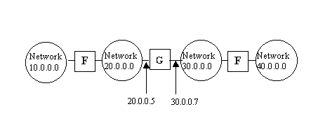
The router (also known as gateway) is a computer that connects between sub-networks (sub-networks represent different logic networks). The routing protocol is located in the network layer. The router’s aim is to route a message (packet) via a sub-network connected directly to it towards its destination.
The routing protocol is “table-driven”, thus each router has a table with entries for each sub-network that exists. The table holds for each entry the name of a destination sub-network and to which adjacent sub-network the router has to pass the message in order to get it to its destination. Also it may contain additional information such as the cost of reaching that destination. The distance is measured in the number of sub-networks on the way (and their speed) and the time spent in each router on that way.
Example:

The Routing Table:
To reach host on network: |
Route to this Address: |
20.0.0.0 |
Deliver directly |
30.0.0.0 |
Deliver directly |
10.0.0.0 |
20.0.0.5 |
40.0.0.0 |
30.0.0.7 |
The router’s algorithm :
Upon receiving a packet:
- Extract destination IP address Id from packet header
- Compute IP address of destination sub-network In
- If In matches any directly connected network send packet to destination
- Else If In appears in the routing table – route as specified in the table
- Else route to default router.
The network will be represented by a graph whose nodes are the routers and the edges are the sub-networks that connect between them.
The trivial problem that this paper deals with is to which adjacent router should the current router send its packet in order to get it as quickly as possible to its destination. In other words: finding an optimal policy for constructing and updating the routing table of each router.
Due to the network large structure and its continuous changes in terms of load and topology, the routing algorithm should be fully distributed, thus able without a central coordinator to disseminate knowledge about the network and find shortest paths on the dynamic network.
Different algorithms for routing packets efficiently over the network will be presented. Each one of the alg., is based on one of the papers that this survey references to.
3. Algorithms
3.1 Belman-Ford algorithm for shortest path on graph
This section discusses the BF algorithm for finding the shortest path on a graph. This algorithm is brought here because it serves as a good starting point for the other algorithms, which are based on reinforcement learning and also have common lines with BF.
3.1.1 Preface
The protocols that refer this algorithm are divided in two:
Another important feature is TTL (time to live): its purpose is to prevent from packets to travel for too long on the network (i.e. packets that were routed wrong due to corrupted tables). Each router decreases this counter when a packet is sent through it. If the TTL counter reaches 0 it is dumped.
3.1.2 The algorithm
The Static case:
Finding the shortest path from node 1 to every node on static networks. Namely the weight of an edge can not change, nor the topology of the network.
Dhi the walk from node 1 to node i containing at most h edges.
dij the weight of the edge (i,j)
Initial:
dij = infinite if (i,j) is not an arc of the graph
Dh1= 0 for all h
D0i= infinite for all i<>1
Step:
for all i<>1
Dh+1i = min{ min j [dij + Dhj] , Dhi }
Termination:
for all i: Dhi = Dh-1i
The algorithm “discovers” at each step at least one node i which the path to it from node 1 is the shortest one. An intuition to correctness of the algorithm is: given that the shortest path to node i is of length n than there must be a node j on this path with length n-1 which is previous to i. Thus by induction node i will be discovered after node j. Hence after at most |V| iterations (the longest path without loops) the algorithm will stop.
The way this algorithm is applied to networks:
Assumptions:
There are no negative loops thus after a node i is “discovered” by the algorithm there can not be a shorter path to it which will be found in the future which now is longer to i. In other words, there is no backward relaxation after a node is disclosed.
For each node i we can keep also the path to it from 1 in addition to the cost.
The Dynamic case:
The problem is when the topology of the network changes or the weight of an edge varies due to dynamic changes in the network as load level.
[DV] In this case the algorithm is modified s.t. each router will send its routing table to its neighbors every period of time (synchronously). Upon receiving a table from a neighbor j router 1 updates its table as follows:
Di = { (min j belongs to N(l)[ d1j + D`i ]) , Di }
where j<>1, N(l) denotes the set of current neighbors of node l and D`i is the value received from node j’s table.
When a router receives a table from its neighbor it will try to minimize its own routing table.
A problem that arises is the slow propagation of network information to other routers. This results due to small traffic of information – only between neighbors.
[LS] Another solution is sending ones routing table to all the other routers of the network. In addition every router will add to which networks it is connected directly. Thus every router would reconstruct in its memory the true structure of the network.
This section will describe a self-adjusting algorithm for packet routing in which a reinforcement learning “module” is embedded into each node. This algorithm uses only local communbetween neighbors in order to keep accurate estimates about the network at each node. The estimates are maintained in each node in a lookup table Q. The final routing policy equals to the collection of all local decisions made by individual nodes (based on their Q table).
3.2.1 Preface
A definition of the routing problem may be: optimally routing packets on a dynamically changing network with unpredictable usage patterns.
The Q-routing alg. presented here, tries to confront this problem. The alg. is a variation of the Q-learning algorithm.
The experiments were carried out using a discrete event simulator. Packets were periodically inserted into the network at random nodes with random destination. In a unit time a router takes the top packet from its queue, examines its destination and decides to which adjacent node to send it to.
3.2.2 The algorithm
The policy decides to which adjacent node to route a packet in order to minimize its whole trip time. Thus the policy’s performance can be measured only after the packet has reached its destination. This way there isn’t any immediate reward to a decision or a possibility to directly evaluating a policy. However using Q-learning ideas the updates of a policy can be made quicker and using only local information that propagates “bottom up” the graph.
Denote: Qx(d,y) - the time node x estimates takes to deliver a packet P, bound for node d, via x’s neighbor node y, including the time spent in node x’s queue.
Algorithm:
y = argminy{ Qx(d,y) + transmission time to y }
t = min z is a neighbor of y Qy(d,z).
Given that P actually spent q units of time in x’s queue and s units in transmission to y, x can update its estimate s.t.:
D Qx(d,y)=a ( q + s + t - Qx(d,y) )
a (alpha) is the usual “learning rate” or “convergence rate” parameter.
This algorithm can be viewed as a version of the dynamic Belman Ford algorithm [DV], since the best path relaxation is made dynamically between neighbor nodes
However unlike dynamic BF:
1.The path length is measured not only by sum on edges but by total delivery time
2.The traffic between nodes is asynchronous and specific (only when a packet arrives and only between a node and its best neighbor).
3.2.3 Results
The algorithm was tested on various network topologies with changing traffic load. The measurements were on the average delivery time of packets, and were compared against the shortest paths algorithm.
Example: test of the Q-routing algorithm against shortest path algorithm:
The network structure: (Irregular grid topology):
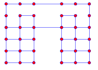
Diagram of a run time result (- showing for each routing policy, how many routing paths go trough each node):
-------Shortest
paths alg. ----------------------------------------Q-routing alg.--------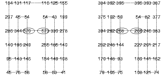
The performance
of Q-routing against shortest paths: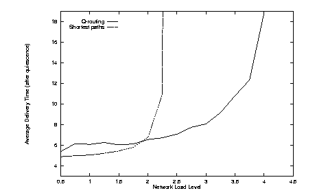
3.2.4 Discussion
The experiments that were carried out on this example regarded these domains:
Topology changes: Connecting and disconnecting nodes from the grid. Q-routing reacted fast to this changes and was able to continue efficiently.
Traffic patterns: Oscillating between 2 patterns that the traffic is directed by (North-South, East-West). Q-routing adapted successfully to each change of directions after a period of adaptation.
Load Level: Under conditions of low network load the algorithm learns to route packets along shortest paths (as BF), after a period of inefficiency during which it explores the network (under low load the optimal policy is shortest paths since no queues exist at nodes).
As network load increases, shortest path routing scheme ceases to be optimal: it ignores the rising levels of congestion on some routers (found on bottlenecks) and floods the network through them. Q-routing adapted its policy to route its packets over new paths thus avoiding the congested bottleneck.
Problems:
This problems are due to the disability of the algorithm to fine tune a policy to discover new shortcuts, since only the best neighbor’s estimate is ever updated. i.e: after a node x learned its best neighbor y to destination d, a neighbor of x, z will become better than y to d. x will never route through it since it already knows its best node y, thus will never get from z its improved estimate to d since it will not send to it nothing. The same will happen if a shorter path arises. This is the drawback of the greedy Q-learning.
Solutions:
3.3 The PQ-routing algorithm (predictive Q-routing)
This section will provide an algorithm that will resolve the problems that were mentioned above for the Q-routing alg..
3.3.1 Preface
As mentioned in [section 3.2.1] the goal is to minimize the total delivery time of a packet in a non stationary environment where each node has no prior knowledge of the environment and only local communication between the neighbor nodes is allowed.
The Q-routing algorithm must regard the tradeoff between exploration and exploitation. Exploration of the “state space” is essential to learning a good policy, however continual exploration without putting the learned knowledge into practice is of no use. This results into dividing the learning into 2 phases: exploration in which actions are selected randomly and exploitation in which the action is selected greedy as the minimum between neighbors of a node.
However the problems that arise from the Q-routing alg. are:
1. Hysteresis problem: the alg. fails to adapt to the new optimal path when load is lowered, because once a longer path is selected, the “minimum selector” is not able to notice decrease in other paths.
2. Q-routing is not able always to find shortest paths under low load. i.e. if there exists a longer path with Q-values less than the shortest path then the alg. will not be able to find shortcuts to the shortest path.
3. Random exploration has negative effects on congestion.
It is possible to mix both phases into one using the epsilon - greedy concept. Thus a probabilistic scheme for choosing next nodes is given which shifts gradually from one phase to the other. However since networks dynamically change (traffic and topology) exploration must be continuous. Hence an algorithm which adapts between the phases is needed.
3.3.2 The Algorithm
The predictive Q-routing algorithm keeps the best experiences (best Q-values) learned and reuses them according to its probabilistic prediction.
Intuition: Under low network load the optimal policy is shortest path routing policy. If load increases the shortest path policy isn’t the optimal since these paths become co. However, if the congested paths are not used for a period of time they will “recover” and become “good candidates”. Therefore the alg. should “probe” those paths at a frequency depending on the congestion level and recovery speed of the path.
TERMS: (D =delta ,a = alpha, b=beta...)
Probing – exploration of potential candidates to be optimal paths
Congestion level – the Q value of a path
Recovery rate-the rate that the congestion of a path changes. It depends only on the current network state thus should be adjusted for every packet sent.
TABLES:
Qx(d,y) – estimated delivery time from x to d via neigbor y
Bx(d,y) – best estimated delivery time from x to d via neigbor y
Rx(d,y) – recovery rate of path x to d via y – is it getting congested or not. (Set negative or zero otherwise it can unlimitedly raise the Q value of a node thus not reaching that node ever)
Ux(d,y)- last update time for path x to d via y.
TABLE UPDATES: (after receiving a packet P,y returns to x its estimate Qy(d,z) )
D Q = [transmission delay + queue time at y + minz{ Qy(d,z)}] - Qx(d,y)
Qx(d,y) ) <- Qx(d,y) + a D Q
Bx(d,y) <- min( Bx(d,y) , Qx(d,y) )
if (D Q < 0) then //path is recovering
D R<- D Q/(current time - Ux(d,y))
Rx(d,y) <-Rx(d,y) + b D R //decrease of R
Else if (D Q > 0) then //path gets congested
Rx(d,y) <-g Rx(d,y) //increase of R
End if
Ux(d,y) <-current time
ROUTING POLICY: (finding neighbor y)
For each neighbor y of x:
D t = current time - Ux(d,y)
Q`x(d,y) = max {(Qx(d,y) + D t Rx(d,y)) , Bx(d,y)}
y =argminy{ Q`x(d,y) }
PARAMETERS:
a (alpha)- Q learning parameter. Set to 1 as to maximize the learning rate.
b (beta)- recovery rate (0.7)
g -(gamma)- decay of the recovery rate which affects the probing frequency (0.9)
As seen the algorithm uses the recovery rate of a path to better estimate its Q value. Thus we can predict the traffic trend on that path and if it congests to find another one, moreover if the alg. predicts other path has recovered, it is “probed”.
Also the algorithm controls all its other “best” paths by keeping Ux(d,y) and Bx(d,y) for each neighbor. Hence PQ will probe paths that have been inactive for long time thus returning to previous best paths.
3.3.3 Results
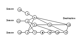
Q-routing policy first sends all the packets along shortest paths - node 4. After it gets congested nodes 12,13 switch to the middle path – node 5. After node 5 gets congested nodes 12,13 switch to the lower path and stay there as long as the load will not increase.
PQ-routing learns the recovery rates and alternate only between the upper and middle paths. Thus returning faster to best paths.
The PQ algorithm deals successfully with the “hysteresis” problem. Namely when a node’s load decreases, PQ is able to utilize the new optimal paths. This is done probing other paths and adjusting Rx(d,y), thus we can predict when its is possible to reuse a path.
Both Q-routing and PQ-routing need an initial period of exploration in which they are non-efficient. However PQ learns a stable policy faster due to the prediction feature – table R. Under increasing high load the alg. adjusted faster and performed better.
3.3.4 Discussion
The PQ-routing algorithm comparing to Q-routing performed better under low, high and varying network load. It adjusts faster to traffic changes by occasionally probing best paths that have been inactive for long time. Moreover the alg. uses predictive learned information about paths, which shortens the adaptation time. Namely – using the recovery rates: D t*Rx(d,y) when updating Q`x(d,y).
If the congestion and load level remains high the PQ alg. will gradually act as Q-routing.
PQ alg. also uses more memory then Q alg.
3.4 The DRQ-routing algorithm (dual reinforcement Q-routing)
3.4.1 Preface
In Q-routing a node’s learning is based on the information received from its neighbor after sending a packet to him. This is called “forward exploration” or forward learning. Thus “backward exploration” is a node’s learning from the information appended to a packet received by it. The scheme that is presented combines the Q-routing algorithm with Dual Reinforcement Learning. The result is the addition of “backward exploration” to the original alg.
3.4.2 The Algorithm
Intuition: When a node x sends a packet P to its neighbor y it can send along some Q value information of node x. Upon receiving the information node y will update its own estimate regarding node x. Thus later on when y will have to make a decision it will have an updated Q value of x.
Denote:
s – the source node of packet P
d – the destination node of P
Qx(z`, s) = minz is a neighbor of x Qx(z,s) //this is the estimated time it takes for a packet destined to node s from node x.
Algorithm:
x sends to y Qx(z`, s) together with packet P
upon receiving a packet y updates its estimate Qy(x, s) of sending a packet to s via x:
D Qy(x,s)=b ( qy + sy + Qx(z`, s) - Qy(x,s) )
Recall that qy is the time spent in y’s queue and sy is the time it takes to send a packet from y to x. b is the (backward) learning rate.
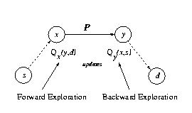
It can be seen that the information about the path that the packet has traversed so far is used to update a Q value of a receiving node.
3.4.3 Results
The experiments that tested the alg., and the simulations were similar to others described before. Measurements were carried out during the learning period to test the learning performance and after the learning settled to test the quality of the final policy. The forward learning rate a was set to 0.7, the backward learning rate b was set to 0.9.
Comparison between performance of Q-routing and DRQ:
3.4.4 Discussion
Exploration and adaptation are 2 terms strongly linked together: the better the exploration, the faster the policy adapts to the network. Hence backward exploration makes adaptation more effective in two ways:
Hence at low load levels DRQ is 3 times faster since it needs little exploration time and its learning is more accurate. At high load levels the accurate learning leads to a better policy.
In backward exploration an additional Q value is appended to the packet, thus increasing the packet size. This is considered to be the backward exploration overhead. Since the ratio of the added size to the average packet size is 0.1%, the additional data is negligible relative to the factor 2 of the improvement of DRQ.
DRQ alg. the same as Q-routing is not able to adapt to decrease of load level and to find short cuts if available. However the PQ-routing could be extended to DRQ easily.
3.5 Q-routing variations and Confidence Intervals alg.
This section will present some variations on the dynamic BF shortest paths alg. and regarding Q-routing. A comparison between Q-routing alg. and these variations will lead into the Confidence interval alg. This algorithm performs better under heavy load at the cost of decreased efficiency under low load.
3.5.1 Preface
We present some experiments done on Q-routing alg. and BF shortest paths in order compare between them. The experiments were performed using a discrete event simulator. packets were inserted at random nodes. Upon receiving a packet a node either added it to the end of its queue or excluded it from the network if it reached its destination. It was assumed that upon receiving a packet, a node sends the “Q update” data to its ancestor instantaneous. Also it was assumed that a node’s queue is unbounded.
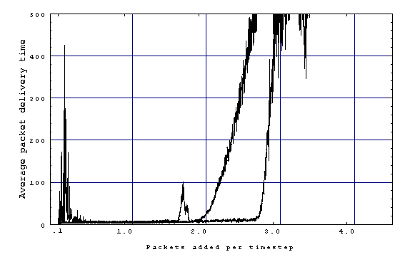
In comparison to the static shortest path alg. the performance of Q-routing was much better. Moreover it was able to sustain a much higher load than shortest path.
It was also observed that at the point that shortest path “blows up”, Q-routing experiences a momentary rise in the avg. delivery time but overcomes it by learning a new policy. This is the result of the greedy property of the alg.: it continuously tries to improve itself.
3.5.2 Variations regarding Q-routing
The idea that an increase in the network information a node receives will lead to better routing decisions is the basis of this alg.
Given that it is possible to relax the queue’s length that a node has into a graph with no queues and with additional directed edges with the weight of the queue (i.e. node x with queue |q| = a will be reduced to an edge e(x,x`) w(x,x`)= a). Note that e(x,x`) constantly changes. Therefore the optimal algorithm will be - dynamic Belman Ford alg. for shortest paths .[section 3.1].
The “best path” alg. will implement a variation of this alg. : at each time step the simulation makes an “all-pairs shortest path” calculation and updates dynamically a global lookup table. I.e. the table will hold for each node s: an entry for each other node t holding the cost to t and through which adjacent s should route).
node s:
Destination
cost
Adjacent node
T
100
Y
Note that this alg. isn’t optimal since paths may change faster than packets are delivered.
The results showed that this alg. sustained high load twice as good as Q-routing.
In order to have the locality constrain of Q-routing in which only local communication takes place (between a node and its neighbors) the “constant pinging “ alg. was developed.
In this alg. at each time step each node receives updates only from its neighbors. These are used for updating each node’s Q-table as in the normal Q-routing alg. This alg. is similar to the dynamic BF alg. with the locality constrain [section 3.1].
The results with this alg. were better than Q-routing due to the fast propagation of information about the network. Thus each node holds better estimates on the network. In comparison with the “full echo” alg. [section 3.2] in the “constant pinging” alg. information propagates constantly whereas in “full echo” it propagates only when processing a packet.
In attempt to limit the amount of communication between neighbor nodes (in order to lower the routing information transmissions) the “variable pinging” alg. was examined.
In this alg. a neighbor node y is queried for its estimate after an amount of time ty has passed since last update.
The results were not much better than the previous alg.
Since Q-routing is greedy it acts to exploit only what it already knows, thus it can return a suboptimal policy by not exploring other “not minimum” neighbors. However other versions of Q-routing as “best paths” or “constant pinging” that do have correct information of the network, increase a lot the congestion of the network while maintaining this information. “Full echo” and “Variable pinging” though not flooding the network with additional data might result in oscillations between their final policies.
Therefore another algorithm was proposed: keeping statistics about the estimates received, thus decisions about exploration are more informed.
3.5.3 The Confidence Intervals algorithm
The idea is that in addition to the estimate of the delivery time, estimates of the confidence of this data is held.
Denotes(regarding some node y):
my(x,d): mean of the sample for past replies from node x for destination d
s y(x,d): standard deviation of the sample
t: Student’s t function
Note: the sample is obtained by keeping a list (moving window) of past replies from x about d.
ly(x,d) = my(x,d) - ta/2n-1 s y(x,d) // the lower bound of the confidence interval
Algorithm (change of Q-routing alg. for some node y):
Thus the algorithm will take a value that is both minimal mean estimate and most stable one. Therefore we make the learning algorithm explore and not “stick“ to a policy as long as the network load changes, or if its “picked” neighbor changes. Thus the exploration phase is not arbitrary but depends on the stability of the network chosen path.
3.5.4 Results
In experiments when the load increased to a value and then settled the Confidence Intervals alg. performance was better than the greedy alg. It was able to sustain a higher load than Q-routing but was slower to learn since its exploration phase is until the network traffic settles. In experiments when the load varied continuously the alg. “stuck” on particular policies.
The results show that though the greedy alg. can be improved, the results received by the more complex Confidence Interval alg. are not worth the overhead.
This chapter will present two distributed algorithms that are based on biologic ants that explore the network and learn good routes. The algorithms confront successfully topology changes and changes in link costs. The algorithms are highly effective under high failure rate and dealing with corrupted router’s data.
3.6.1 Preface
The problem involved in routing over dynamically changing networks is the dynamics: the random network topology changes and the changing link cost due to congestion and load. Another problem is corrupted data in routers. The learning algorithms that are brought here confront successfully with these problems. They are inspired by the dynamics of how ant colonies learn shortest paths using little space and time in their computation. The algorithms are: “regular ant alg.” which returns a single shortest path, and “uniform ant alg.” which returns multi-shortest paths.
3.6.2 The Algorithms
Denotes:
Host: communication endpoints – they initiate or terminate data packets.
Routers: nodes that forward data.
Ants (that explore the network): Messages that are periodically generates by hosts hd to randomly chosen host destination hs. An ant structure is: (hd,hs,c). c is the cost sending a message from hs to hd . It is initialized to 0 and each router that the ant reaches increments c s.t. it reflects the cost of the inverse path it has traveled (i.e. on a path a->b, c will reflect the cost b->a). Thus ants explore paths backward from destination d to source s.
Probabilistic routing tables: router r maintains for each destination x an entry in its table of the form r: ( x,(y1,p1),(y2,p2), …,(yn,pn) ) where for all i, yi is neighbor of r. Sum {pi }= 1. Upon r receiving a packet destined to x, r forwards it to its neighbor yi with probability pi.
Probabilistic updates of routing tables by ants: An ant will update the routing tables of all routers on its way similar to Q-routing but in a non-linear way:
Algorithm:
Upon r receiving an ant (hd,hs,c) on link li from yi then:
r updates c with the cost of traversing li in reverse.
r updates the entry for hd (hd ,(y1,p1),(y2,p2), …,(yn,pn) ) as follows:
pi = pi+D p/1+D p ; pj = pj/1+D p 1<= j<= n , i<>j
D p = k/f(c) k>0 , f(c) is a non-decreasing function of c.
k is the learning rate (<0.1). k has to be big enough that each arriving ant has an effect on pi and small enough that the algorithm converges.
In this way an entry in the routing table will reflect for each neighbor of r yi: how congested is the path through yi to hd. Hence receiving a packet from yi means that the path to hd via yi is active and the alg. will raise its valuproportionally to its cost c.
Upon r forwarding the ant (hd,hs,c) after updating entry hd:
r uses its routing table entry for hs (hs ,(y1,p1),(y2,p2), …,(yn,pn) ) as follows:
r forwards the ant to yi s.t.:
yi = argmax j{Pr(ant sent to yj)}
Thus regular ant alg. uses the routing table to forward ants to less congested routes. There is no exploration of less favorable routes. Hence, the algorithm will converge to a single shortest path in the end.
r forwards the ant to any node yi with equal probability
Thus the uniform ant alg. explores all paths equally.
Uniform ant alg. is not prone to route oscillation problems that single shortest path algorithms have due to their greedy property. Due to uniform exploration the alg. will settle down finally on a stable policy while a greedy alg. might converge into 2 “best paths” and continuously oscillate between them.
Uniform ants have a simpler structure than regular ants (hd,c), since they don’t require a destination hs, due to their uniform exploration of the network. However each ant will have a TTL (time to live). This is a major advantage since it allows easy scalability of the network: no node has to know about all the hosts that exist.
3.6.4 Discussion
An analysis of the algorithms proves that both algorithms converge at t® ¥ to a certain policy, however the Regular Ant alg. must be applied to symmetric networks (undirected). The proof is based on analysis of the non-stationary, discrete-time, Markov chain equations that are obtained from the algorithm.
Thus the forwarding probabilities converge to 0 and 1 in each entry in the routing tables. If there are topology changes or link cost changes after convergence, the regular ant policy will not adapt to the new situation since it “does not explore any more”. Uniform ants are immune to this problem since they explore all paths. The adaptation rate depends on k- the learning rate.
Improving the adaptiveness of the regular ant alg. is done applying the e -greedy concept: a router will route regular ants randomly a percentage of the time (e ) and the rest of the time (1-e ) according to the alg..
In general the ant algorithms presented do not need large space in each router’s state, however the overhead is in the increased routing message traffic. However the ants messages are constant and small they can be piggybacked on data packets. On high bandwidth networks this makes the alg. nearly for free in traffic terms.
3.6.3 Results
The experiments were done in order to evaluate the algorithm performance relatively to the link state (LS) alg., distance vector (DV) [section 3.1.1] and Q-routing [section 3.2].
The simple network topology that was used is:
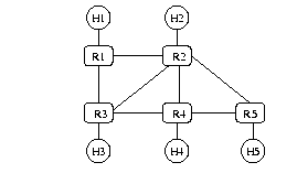
All links are of equal cost 1. The simulation ran a period of time that allowed the algorithms to stabilize themselves. Each host Hi generated ants with a steady frequency. Changes in topology and load were simulated by eliminating links and changing the packet insertion rate.
Uniform ants alg. performed as good as DV and LS in terms of average delivery time. The regular ants alg. with the improvement of e -greedy was slower in adapting to changes. It is also noticed that since uniform ants find multiple paths, the traffic is somehow split between them hence an increase in the available bandwidth is gained.
In terms of amount of traffic generated the ant algorithms exceed those of LS and DV.
The algorithms were tested against the situation of router’s corrupted internal data. Hence a router’s data failure was simulated. With LS the recovery period is bounded by the periodic broadcast interval. With DV the recovery time is bounded by the propagation of the information about the failure. During recovery time the routers are unable to calculate correct routes which may result in routing loops. The ants algorithms perform better under such an event due to the ants backward “walk” and the independent update of each router’s table along this walk.
In comparison with Q-Routing:
This paper presented various approaches and algorithms towards routing packets over dynamic networks with the view of reinforcement learning.
The major work on this field was done around the Q-learning concept, which fitted the structure of the network with routers. The Q-routing algorithm had a primary phase in which it learned the network and afterwards generated a routing policy. The learning was done by propagation of correct estimates from one node to its neighbor. In its second phase the algorithm either acted greedy or e -greedy resembling with the SARSA algorithm.
The problems that the various algorithms confronted are: changes of topology and changes of network load, corrupted router’s data, exploration vs. exploitation, rediscovering shortest paths after settling on a policy, increasing the learning speed thus shortening the adaptation and exploration time, estimating the exact needed exploration time, learning a routing policy based on the probability of congestion on paths and minimizing the overhead in routing traffic information and routers states that the algorithms consume.
There were some “common” concepts that reappeared with some changes in some of the algorithms such as: Dual Reinforcement learning and Backward exploration (Ants alg. and DRQ alg.), predictive decisions: based on a packet that arrives through a neighbor other neighbors estimates are updated upon predictive parameters. (PQ alg. and Ants alg.), and the e -greedy notion to define the length of the exploration period.
Options to research, improvement and future work based on the mentioned algorithms are:
Replacing the Q-table based representation of the routing policy with a function approximator such as the one used for neural networks. Thus the algorithm could integrate more system variables into each routing decision. On this basis working on a neural network model instead of a HMM could allow more information to be referred and more states defining the network.
Based on the model of TD(g ) it is possible to implement Q-routing as a Q-learning algorithm but instead of updating only from next step’s estimate, the algorithm would take g states lookup and update using those values weighted. Although this could result in an increase in routing transmission between nodes it may improve the convergence rate into a policy and faster propagate changes into the network.
5. References
[1] J. A. Boyan & M. L. Littman (1993). A distributed reinforcement learning scheme for network routing. CMU-CS-93-165
[2] J. A. Boyan and M. L. Littman(1994). Packet routing in dynamically changing networks: A reinforcement learning approach
[3] S.P.M. Choi & Dit-Yan Yeung. Predictive Q-routing: A memory-based reinforcement learning approach to adaptive traffic control.
[4] S. Kumar & R.Miikkulainen(1997). Dual reinforcement Q-routing: An on-line adaptive routing algorithm.
[5] J.W. Bates(1995). Packet routing and reinforcement learning: Estimating shortest paths in dynamic graphs.
[6] D. Subramanian, P. Druschel & J. Chen. Ants and reinforcement learning: A case study in routing in dynamic networks.