Finding the Optimal Policy: Value Iteration

In this section we present the Value Iteration algorithm (also referred to as VI) for computing an $\epsilon$-optimal policy^6.1 for a discounted infinite horizon problem.
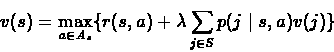
In Lecture 5 we showed that the Optimality Equations for discounted infinite horizon problems are:

$$\begin{eqnarray*}v(s) = \max_{a \in A_{s}}\{r(s,a) + \lambda\sum_{j\in S}p(j\mid s,a)v(j)\} \end{eqnarray*}$$

We also defined the non-linear operator L:

$$\begin{eqnarray*}L\vec{v} = \max_{d\in \Pi^{MD}}\{\vec{r}_{d} + \lambda P_{d}\vec{v}\} \end{eqnarray*}$$

For which it was shown, that for any starting point $\vec{v}_{0}$, the series $\{\vec{v}_{n}\}$ defined by $\vec{v}_{n+1}=L\vec{v}_{n}$, converges to the optimal return value $\vec{v}_{\lambda}^{*}$.
The idea of VI is to use these results to compute a solution of the Optimality Equations. The VI algorithm finds a Markovian stationary policy that is $\epsilon$-optimal.